Grid Algorithm

Over the past couple of weeks, I’ve been writing a small lexer in Rust, motivated by the need for something simpler and easier to use than the default lexer offered by LALRPOP. The in-built lexer allows for simple regexes, but managing these regexes becomes difficult for more sophisticated situations such as double-quoted literals.

The core idea behind a lexer is to convert a stream of characters into a stream of tokens. Each token constitutes a distinct building block that can be used to construct a grammar for a language parser. As an analogy, the vocabulary and punctuation supporting the English language constitute a set of tokens. Of course, you could avoid the lexer altogether and deal directly with the underlying characters, but that makes the language grammar exponentially more complex to specify. Imagine parsing English sentences based on rules associated with each character of the alphabet!

How It Works

To recap, a lexer’s job is to convert a stream of characters into a stream of tokens. Tokens can be anything that’s useful to feed into your parser. The parser is generated from a set of productions declared in a grammar file. LALRPOP provides a bottom-up LR(1)1“LR(1)” expands to a left-to-right, rightmost derivation parser with a single token lookahead. parser. A bottom-up parser uses recognized tokens to construct leaf nodes of the parse tree. In contrast, a top-down parser (of which recursive-descent parsers are the most common) generates productions eagerly as matching symbols are encountered. Top-down parsers are often very convenient and easy to use, but they’re less flexible compared to bottom-up parsers, and require backtracking when they encounter production dead-ends.

One way to structure the lexer is to break it down into a number of processors, one per type of token that you could potentially produce. For example, a Sym processor processes symbols, which are arbitrarily long consecutive sequences of characters conforming to a class (such as letters, numbers and underscores). The processor abstraction is useful for encapsulating logic associated with each token type into its own implementation. The idea is to iterate through each character in the stream, and feed it to each of the processors until one of them accepts the character. If none of the others accept the character, the Err processor is sure to do so (which means the character stream is ill-formed).

This abstraction is represented by the following trait:

pub trait Processor {
    fn accept(
        &self,
        idx: usize,
        chr: Option<&char>) -> Result<LexRes, LexErr>;
}

To complete this definition, the associated types LexRes and LexErr are provided below. The lexer — when fully or partially successful — returns an ordered set of tokens, where each token declares the starting index of the token (relative to the original character stream), the length of the stream consumed, and the type of token (represented by the Cat enum). Notice that some of these enum values such as Sym (for ‘symbol’) and Lit (for ‘literal’) capture a value, whereas others do not.

#[derive(Debug, Eq, PartialEq)]
pub struct LexRes {
    pub tokens: Vec<Token>,
    pub accepted: usize,
    pub rejected: bool,
}

#[derive(Debug, Eq, PartialEq)]
pub struct LexErr {
    pub idx: usize,
    pub msg: String,
}

#[derive(Debug, Eq, PartialEq)]
pub struct Token {
    pub idx: usize,
    pub len: usize,
    pub cat: Cat,
}

#[derive(Clone, Debug, Eq, PartialEq)]
pub enum Cat {
    Sym(String),
    Lit(String),
    Assgn,
    Eql,
    SemiColn,
    LParen,
    RParen,
    Spc,
}

What the simple definition of LexRes above belies is its underlying flexibility. When a processor receives a character, it can choose from 3 options:

  1. Accept k outstanding characters (accepted = k; k ≤ n)
  2. Reject all characters not accepted (rejected = true; k < n)
  3. Wait for more characters (rejected = false; k < n)

The number n represents the total number of outstanding characters, which increments on every iteration, but decrements on acceptance or rejection of characters. Notice that these options are not mutually exclusive; in fact, the first option combines with either the second or third, but the latter cannot be combined with each other.

When the processor chooses the third option, this acts as a signal to the lexer that the next character should be fed directly to this processor. In essence, the processor holds an exclusive lock over the remainder of the stream as long as characters remain pending (neither accepted nor rejected). This process can continue ad infinitum, or at least until the end of the character stream. In each iteration, the processor has the choice of accepting up to the total number of outstanding characters (in stream order), and either rejecting the rest (which ends the cycle and releases the exclusive lock) or continuing to wait for additional characters.

The declared ordering of processors has functional significance in certain situations. For instance, if you have a choice of detecting one of <, - and <- as different token types, you’d likely want the latter to have precedence. Also, as a trivial example, the Err processor is always used as the last resort.

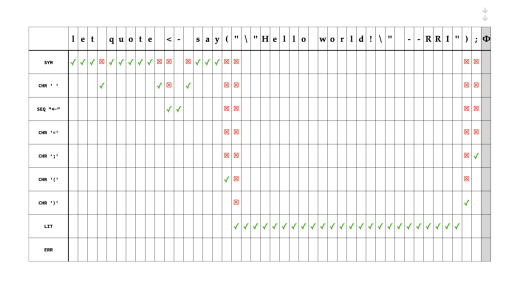
Play the short animation below, for a concrete visual of what the lexer’s processing looks like for the simple character sequence:

let quote <- say("\"Hello world!\" --RRI");

In the example above, let, quote and say are interpreted as symbols using the Sym processor. The Seq processor looks for a specific sequence of characters (here, it is <-, mapping to Cat::Assgn). The Lit processor is distinctive because it internally tracks state associated with the escape character \, which can escape double-quotation marks inside a double-quoted literal.

Complexity

If we assume that (a) we have a small constant number of processors and (b) each processor performs its task in constant time, the overall algorithm is clearly O(n) in time-complexity, with respect to a character stream of length n. However, we can also evaluate how efficient the algorithm is with respect to a baseline. In theory, the only way for us to be certain that a character is part of a particular token is for its processor to accept it, which means that every character must be processed at least once, giving us a total of n processing calls as the ideal minimum to baseline our algorithm against.

From the visual above, it’s clear that the checkmarks (✓) represent the ideal path, whereas the crosses (☒) represent ‘misses’, or distance traveled before the character is accepted. Further, when a processor like Sym rejects the character immediately succeeding its final character (such as whitespace or punctuation, which is not part of the symbol), processing is restarted at the rejected character from the first processor, which, in the particular example, is again Sym. That means we have an extra character to be processed for every symbol recognized (note that ‘symbol’ in this context means the output token of the Sym processor such as let, quote and say). The efficiency of the algorithm with respect to the baseline can therefore be defined as:

\frac{count(\texttt{accept})}{count(\texttt{accept}) + count(\texttt{reject}) + count(\texttt{symbol})}

In essence, this is a number in (0, 1] that is the inverse of the average number of steps until a character is accepted by a processor. It varies based on the string processed by the lexer, so we’d likely only care about average statistics. Applying it to the example above gives us an efficiency of approximately 0.59: on average it takes 1.7 steps for each character to be accepted by a processor. Turning this into a useful metric would require us to normalize it, which we won’t attempt to do today.

Finally, there are further opportunities for refinement. First, each processor requires a different number of character comparisons to complete its task. Although we’ve assumed that each operates in constant time, we really ought to weight each processor, or otherwise measure the total number of comparisons directly. This would give us a more accurate metric than the one presented above. Second, we can order processors to maximize efficiency, basing the order on predictions that we derive from the statistics of the input being processed. We’re still bound by the need to process each character at least once, but we might be able to get really good at predicting which processor to try next, giving us an efficiency of close to 1.

That’s all for today, folks! 🖖

ChaosDB Vulnerability

This is commentary on work done by the Wiz Research Team published here. You should read that article carefully before continuing. I was motivated to write this post because I felt like the incident provided a great example of how the theory of security best practices in software development related to the ground reality of how attackers infiltrate systems.

Trust Minimization

Bug #1 was the entry point to the attack: users were permitted to execute arbitrary C# code as root on Jupyter notebooks. This was probably a configuration error, judging by the fact that users otherwise executed coded as cosmosuser. There are two key takeaways from this point:

(1) Configuration errors are common in practice. Despite our best efforts to have zero errors, we can expect that in a sufficiently complex system, some errors will always creep in. Security best practices therefore have to operate in the context of a reality where errors permeate the system and parts of the system can break at any point. It is not enough to try to prevent errors; it is vital that we detect problems quickly and design the system in a way that limits the blast radius when things break.

Zero Trust is a term that refers to the extreme version of the same idea. In the security realm, trust is a bad thing: it means we expect the object of our trust to operate without error, which deviates from the reality we see around us (note that intentions don’t matter). We can avoid taking an ideological stance on this subject by accepting that if we want to build a robust system, we need to ensure that parts of the system don’t trust each other unless reasonably necessary.

(2) Systems that allow execution of arbitrary code most likely allow execution of arbitrary actions. This might seem like a tautological statement but it has deeper meaning. On one side of the equation, software developers might see arbitrary code execution systems as the epitome of loose coupling, a desirable property of the system. It means that parts of the system don’t need to know about each other, and can evolve mostly independently. On the other hand, no one really wants to allow arbitrary code to be run, because that would mean allowing the system to be taken over (for example, allowing operating system files to be modified).

In reality, we have a common objective of allowing the user of the system to perform specific authorized actions while limiting all others, though it’s not always clear ahead of time what actions need to be authorized. Our choices are (a) to identify what actions need to be authorized and allow just those, or (b) to identify what actions should be considered unauthorized and disallow just those. When people talk about supporting arbitrary code execution, they are, in fact, choosing (b) over (a) at some level within the virtual machine stack.

The trouble with approach (b) is that every level is ridden with errors and escape hatches, and it is rather difficult to plug all the holes, or even be aware of them in the first place. It may be best to avoid designing systems of this kind.

Blast Radius

Bug #2 allowed the root user to bypass firewall rules and gain access to forbidden network destinations. The problem with the configuration was that these firewall rules were set up on the Jupyter notebook container itself. As the article points out, a better alternative would have been to enforce these rules outside the Jupyter notebook container. This example demonstrates the importance of designing the system with a keen understanding of blast radius. A typical design process might start by asking:

Q1. Is network access restricted?
A1. Yes, via iptables rules.
Q2. Can a user bypass the iptables rules?
A2. No, they have to be root for that.

In practice, good security design needs to consider additional questions. For instance:

Q3. If the user becomes root, can we still limit the damage?
A3. Yes, we can implement the control outside the container.

It is often helpful to think of these controls as defenses. Defenses are designed to be robust, but they are not perfect, and can fail under clever and sustained attacks. When defenses fail, the system is weakened of course, but shouldn’t fail catastrophically. In parallel, failure of defenses should be monitored, and quick action should be taken to fortify the system.

Least Privilege Principle

Later on, the article points out another example of unexpectedly large blast radius:

“…we expected to get two keys: a private key and a public key used to encrypt and decrypt the protected settings. […] In reality, we got back 25 keys.

Could the impact have been reduced? For one thing, it isn’t clear if the service truly needed to vend all 25 keys to all clusters. It may also have been judicious to create distinct secrets for distinct purposes, and provide access to only the ones that the particular sub-system needed to do its job correctly. It’s easy to get lazy and assume that there is an ‘administrator’ with global access and super-powers, but this is recipe for disaster in a world where mistakes are inevitable.

Security Through Obscurity

The researchers were able to query a ‘certificates’ endpoint to fetch the secrets needed to intercept and gain access to hundreds of customer accounts. One aspect of this attack I’d call out is how easy it was for them to disassemble the WindowsAzureGuestAgent.exe file, and discover the certificate package format. This is something that software developers need to keep in mind as they develop robust software: the security of the system should never be contingent on attackers’ ignorance of system behavior or other knowledge (besides cryptographic secrets).

That’s all for today, folks! 🖖

From Fixed Points to Recursion

Recursion refers to self-referential code. Most people are familiar with recursion in the form of names that are used before their values are fully computed. The classic Fibonacci function can be used to illustrate this. As you can see, the definition of fib references itself.

fib :: Int -> Int
fib 0 = 0
fib 1 = 1
fib n = fib (n - 1) + fib (n - 2)

The fix function in Haskell calculates the least fixed point of the function provided as argument, if it exists. From numerical analysis, you may recall a fixed point as a value at which the output remains unaltered no matter how many times you apply the function to it. In other words, the following statement is true for all f, for which the fix function can be computed:

f (fix f) = fix f

To use the fix function, we first need to a redefine fib as a function that can be supplied to it. We define a new variable f that represents the Fibonacci function, moving fib over to the right side.

let f = \fib -> \n -> if n < 2 then n else fib (n - 1) + fib (n - 2)

In plain English, you could read this as: given the Fibonacci function and a number, we can calculate the value as (a) the number itself if it is less than 2, or (b) the sum of the Fibonacci function applied to the previous two numbers respectively.

Notice that the definition above no longer uses recursion; it simply accepts fib and n as arguments, and calculates the result.

We now find the least fixed point for the Fibonacci function, and apply it to the desired input. For instance, to find the 11th Fibonacci number, we write:

import Data.Function (fix)
fix f 11

…and voila! it prints the result 89.

If you open up the source code of fix, this is how it is defined:

fix :: (a -> a) -> a
fix f = let x = f x in x

Again, in plain English, replace x with the supplied function f applied to (f applied to (f applied to (…))), then return x. You would think this would go into an infinite loop — and it does, if the function doesn’t converge — but it actually works! One of the advantages of a language with non-strict evaluation semantics like Haskell is the ability to work effectively with infinite regress.

Link to GitHub

That’s all for today, folks! 🖖